Thousands of programming languages were invented in the first 50 years of the age of computing. Many of them were similar, and many followed a traditional, evolutionary path from their predecessors.
But some revolutionary languages had a slant that differentiated them from their more general-purpose brethren. LISP was for list processing. SNOBOL was for string manipulation. SIMSCRIPT was for simulation. And APL was for mathematics, with an emphasis on array processing.
What eventually became APL was first invented by Harvard professor Kenneth E. Iverson in 1957 as a mathematical notation, not as a computer programming language. Although other matrix-oriented symbol systems existed, including the concise tensor notation invented by Einstein, they were oriented more towards mathematical analysis and less towards synthesis of algorithms. Iverson, who was a student of Howard Aiken’s, taught what became known as “Iverson Notation” to his Harvard students to explain algorithms.
Iverson was hired by IBM in 1960 to work with Adin Falkoff and others on his notation. In his now famous 1962 book “A Programming Language” 1 , he says the notation is for the description of “procedures…called algorithms or programs”, and that it is a language because it “exhibits considerable syntactic structure”. But at that point it was just a notation for people to read, not a language for programming computers. The book gives many examples of its use both as a descriptive tool (such as for documenting the definition of computer instruction sets) and as a means for expressing general algorithms (such as for sorting and searching). Anticipating resistance to something so novel, he says in the preface, “It is the central thesis of this book that the descriptive and analytical power of an adequate programming language amply repays the considerable effort required for its mastery.” Perhaps he was warning that mastering the language wasn’t trivial. Perhaps he was also signaling that, in his view, other notational languages were less than “adequate”.
The team, of course, soon saw that the notation could be turned into a language for programming computers. That language, which was called APL starting in 1966, emphasized array manipulation and used unconventional symbols. It was like no other computer program language that had been invented.
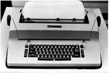
APL became popular when IBM introduced “APL\360” for their System/360 mainframe computer. Unlike most other languages at the time, APL\360 was also a complete interactive programming environment. The programmer, sitting at an electromechanical typewriter linked to a timeshared computer, could type APL statements and get an immediate response. Programs could be defined, debugged, run, and saved on a computer that was simultaneously being used by dozens of other people.
Written entirely in 360 assembly language, this version of APL took control of the whole machine. It implemented a complete timesharing operating system in addition to a high-level language.
With the permission of IBM, the Computer History Museum is pleased to make available the source code to the 1969-1972 “XM6” version of APL for the System/360 for non-commercial use.
The text file contains 37,567 lines, which includes code, macros, and global definitions. The 90 individual files are separated by ‘./ ADD” commands. To access this material, you must agree to the terms of the license displayed here, which permits only non-commercial use and does not give you the right to license it to third parties by posting copies elsewhere on the web.
Jürgen Winkelmann at ETH Zürich has done an amazing job of turning this source code into a runnable system. For more information, see MVT for APL Version 2.00.
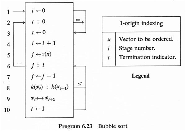
Iverson’s book “A Programming Language” 1 uses a graphical notation that would have been difficult to directly use as a programming language for computers. He considered it an extension of matrix algebra, and used common mathematical typographic conventions like subscripts, superscripts, and distinctions based on the weight or font of characters. Here, for example, is a program for sorting numbers:
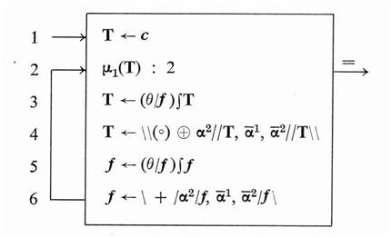
To linearize the notation for use as a computer programming language typed at a keyboard, the APL implementers certainly had to give up the use of labeled arrows for control transfers. But one feature that they were able to retain, to some extent, was the use of special symbols for primitive functions, as illustrated in this program that creates Huffman codes:
APL uses symbols that are closer to standard mathematics than programming. For example, the symbol for division is ÷, not /. To support the unconventional symbols, APL\360 used a custom-designed keyboard with special symbols in the upper case.
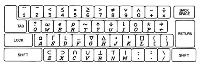
APL\360 used a custom-designed keyboard
Even so, there were more special characters than could fit on the keyboard, so some were typed by overstriking two characters. For example, the “grade up” character ⍋, a primitive operator used for sorting, was created by typing ∆ (shift H), then backspace, then ∣ (shift M). There was no room left for both upper- and lower-case letters, so APL supported only capital letters.
For printing programs, Iverson and Falkoff got IBM to design a special type ball for their 1050 and 2741 terminals, which used the IBM Selectric typewriter mechanism.
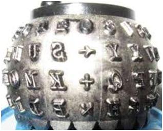
Now programs could be both typed in and printed. Here, for example, is the printed version a program from the APL Language manual 2 that computes the mathematical determinant of a matrix:

APL is a concise high-level programming language that differs from most others developed in the 1960s in several respects:
Order of evaluation: Expressions in APL are evaluated right-to-left, and there is no hierarchy of function precedence. For example, typing the expression
2×4+3
causes the computer to immediately type the resulting value
14
The value is not, as in many other languages that have operator precedence, 11. Of course, parentheses can be used to group a subexpression to change the evaluation order. The general rule is that the right argument of any function is the value of the expression to its right.
Automatic creation of vectors and arrays: A higher-dimensional structure is automatically created by evaluating an expression that returns it, and scalars can be freely mixed. For example,
A ← 2 + 1 2 3
creates the vector “1 2 3”, add the scalar 2 to it, and creates the variable A to hold the vector whose value is
3 4 5
Variables are never declared; they are created automatically and assume the size and shape of whatever expression is assigned to them.
A plethora of primitives: APL has a rich set of built-in functions (and “operators” that are applied to functions to yield different functions) that operate on scalar, vectors, arrays, even higher-dimensional objects, and combinations of them. For example, the expression to sum the numbers in the vector “A” created above is simply
+/A
where / is the “reduction” operator that causes the function to the left to be applied successively to all the elements of the operand to the right. The expression to compute the average of the numbers in A also uses the primitive function ρ to determine how many elements there are in A:
(+/A) ÷ ρA
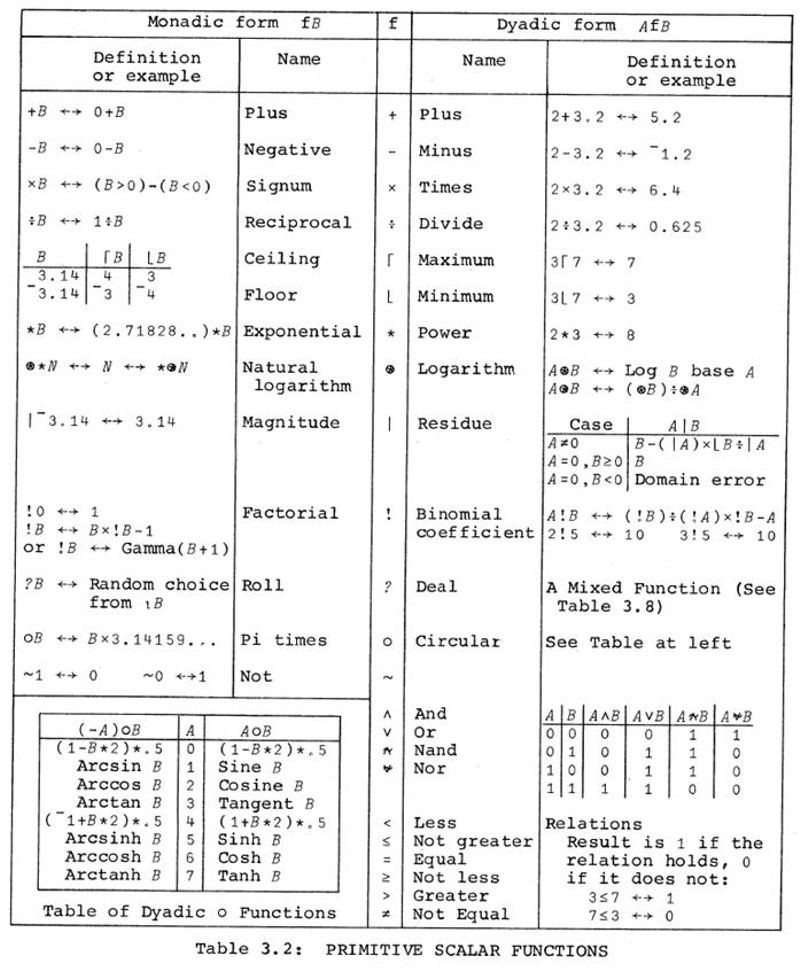
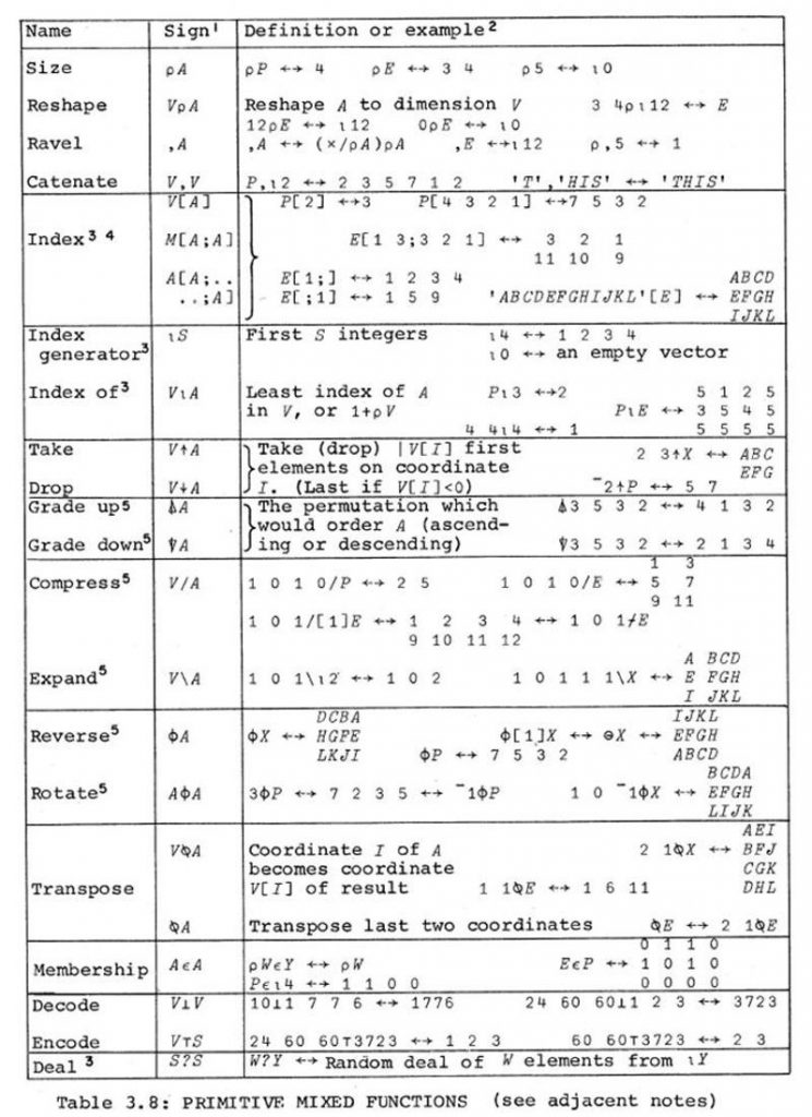
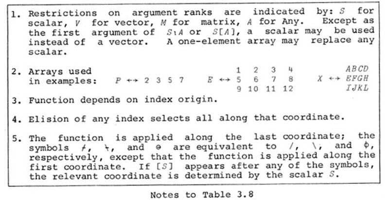
Here are some tables from the 1970 “APL\360 User’s Manual” 3 that give a flavor of the power and sophistication of the built-in APL functions and operators.
APL encourages you to think differently about programming, and to use temporary high-dimensional data structures as intermediate values that are then reduced using the powerful primitives. A famous example is the following short but complete program to compute all the prime numbers up to R.
Here is how this expression is evaluated:
subexpression
meaning
value if R is 6
Generate a vector of numbers from 1 to R.
Drop the first element of the vector and assign the rest to the temporary vector T.
T∘.×T
Create the multiplication outer product: a table that holds the result of multiplying each element of T by each element of T.